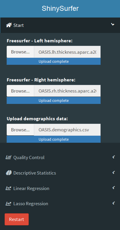
Load .txt files created by FreeSurfer using the aparcstats2table command for the left and right hemisphere. In these files each line represents an individual participant and each column represents the mean value for a cortical area (cortical thickness, volume, area, or curvature). At present, ShinySurfer only accepts data files based on the brain parcellation developed by C. Destrieux et al. (Neuroimage 2010;53:1-15). You may also load a .csv file containing additional information for each participant, such as sex, age or clinical information. Example datasets can be found at GitHub.

The data order of the columns is ID, sex, age. The remaining columns are 74 regions of the left hemisphere and 74 regions of the right hemisphere. All column names must exist, but related data can be null. In this OASIS data set, there are 300 data sets in total.

After the data has been loaded, the following functions are available: Quality Control with Raincloud Plots, Descriptive Statistics with the Brain Map, Linear and Lasso Regression. You can filter the columns and information as you wish. To restart the Shiny App use the Restart-Button.
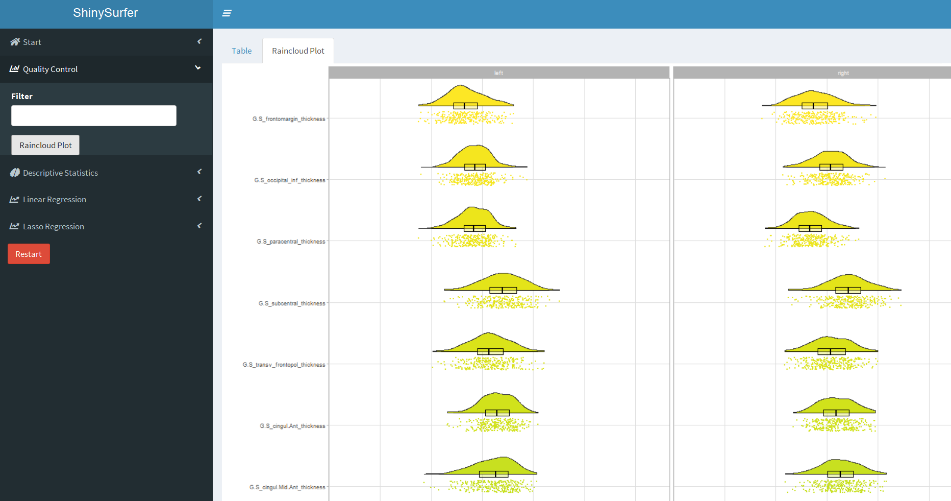
The data files are combined and displayed as one table on the right. In the table you may sort all variables in ascending or descending order by clicking on the small arrows after each variable name. After clicking on Raincloud Plot, ShinySurfer produces raincloud plots for all cortical areas in a new tab based on code provided by M. Allen et al. (Wellcome Open Res 2021;4:63). The raincloud plots combine a dot plot of raw data, a plot of probability density, and a box plot, showing the median and the quartiles. Before creating raincloud plots, you may filter your dataset based on every variable in the table to display subsets of your data.
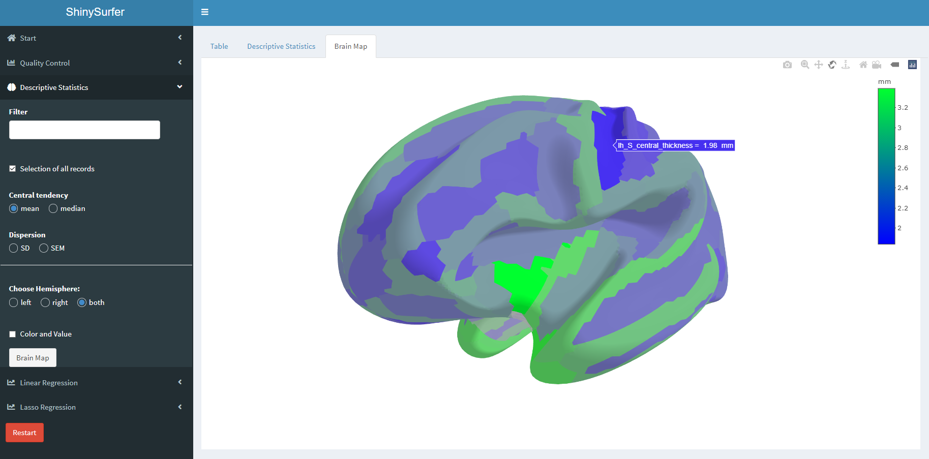
After clicking on Brain Map, ShinySurfer displays the central tendency (mean or median) or dispersion (standard deviation or standard error of the mean) on a semi-inflated 3D standard brain using code provided by A. Mowinckel et al. (Adv Methods Pract Psychol Sci 2020;3:466-483). When you move the pointer inside the Brain Map tab, a toolbar appears in the right upper corner, allowing you to zoom, pan, and rotate the brain model. Before creating the 3D brain map, you may filter your dataset based on every variable in the table to display subsets of your data.
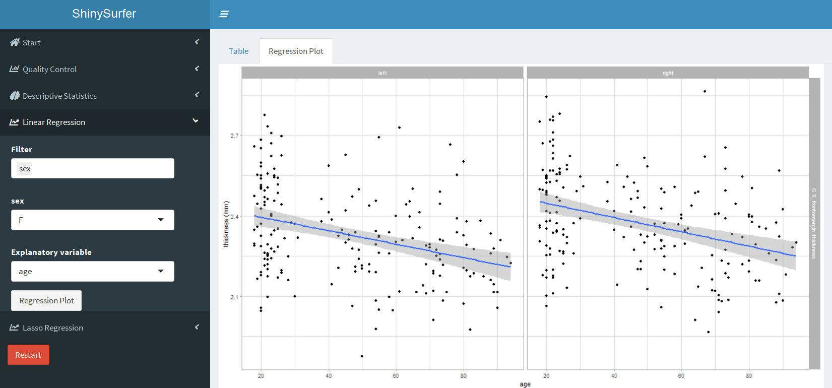
After clicking on Regression Plots, ShinySurfer creates scatter plots for every cortical area with the cortical parameter on the y-axis and the chosen explanatory variable on the x-axis. ShinySurfer also displays the linear regression line and the 95% confidence interval of the regression line.
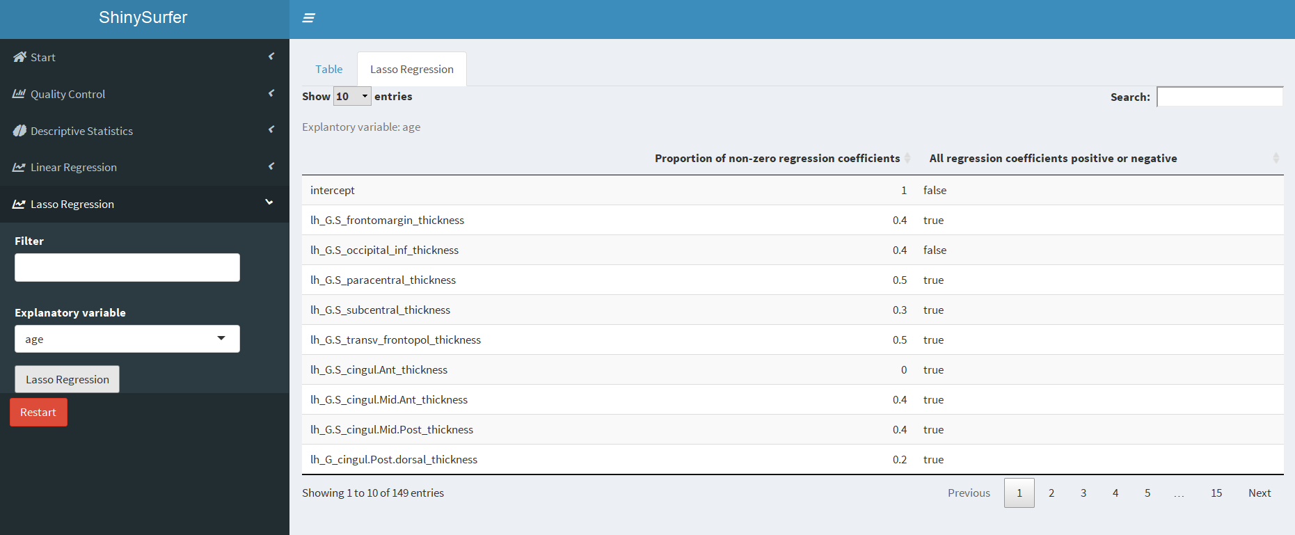
ShinySurfer is able to perform a bootstrapped lasso (least absolute shrinkage and selection operator) regression analysis for variable selection (Tibshirani 1996). After choosing the explanatory variable and clicking on Lasso Regression, ShinySurfer creates a table containing all cortical areas. The table lists the proportion of all non-zero regression coefficients after 1000 bootstraps. In addition, the table states if all regression coefficients for a given cortical area were positive or negative (true).
